This is a re-posting of the wrap-up article which appeared on the IYL2015 main blog.
2015 has been the International Year of Light.
As astronomers, here at the Sloan Digital Sky Survey everything we do is based on collecting light from cosmic objects. So we have been pleased to celebrate the International Year of Light, and especially the Cosmic Light Theme, supported by the IAU. As a small contribution to this celebration, every month in 2015 SDSS had a special blog post talking about the different ways we use light. Here’s a roundup of what we talked about through out the year.
In January we talked about How SDSS Uses Light to Study the Darkest Objects in the Universe. This blog post, by Coleman Krawcyzk and Karen Masters (both from the University of Portsmouth in the UK) with help from Nic Ross (Royal Observatory, Edinburgh) was about finding black holes by looking at the light from distant galaxies. Finding objects which are famous for not emitting any light, using light seems contradictory, but this article explains how the light created by the hot material falling onto a black hole can make these objects outshine the entire galaxy they live in.

An artist’s rendition of a quasar created by Coleman Krawczyk (ICG Portsmouth). The image is drawn on a radial log scale with the central black hole 1 AU in size.
In February we wrote about How SDSS Uses Light to Measure the Distances to Galaxies. This of course was about the technique of measuring galaxy redshifts (ie. the shift of their light to longer wavelengths caused by the expansion of the Universe) by looking at absorption and emission lines in galaxy spectra and comparing their wavelength to the laboratory measurement. Edwin Hubble, and others, realised over 80 years ago, that this can be used to give distances to galaxies, as the amount of redshift increases with the galaxy’s distance. The original motivation for SDSS (back in the 1990s) was to used this technique to measure distances to a million galaxies, and in SDSS-IV we are continuing to use this in the eBOSS part of the survey, to map distances to ever more distant galaxies.

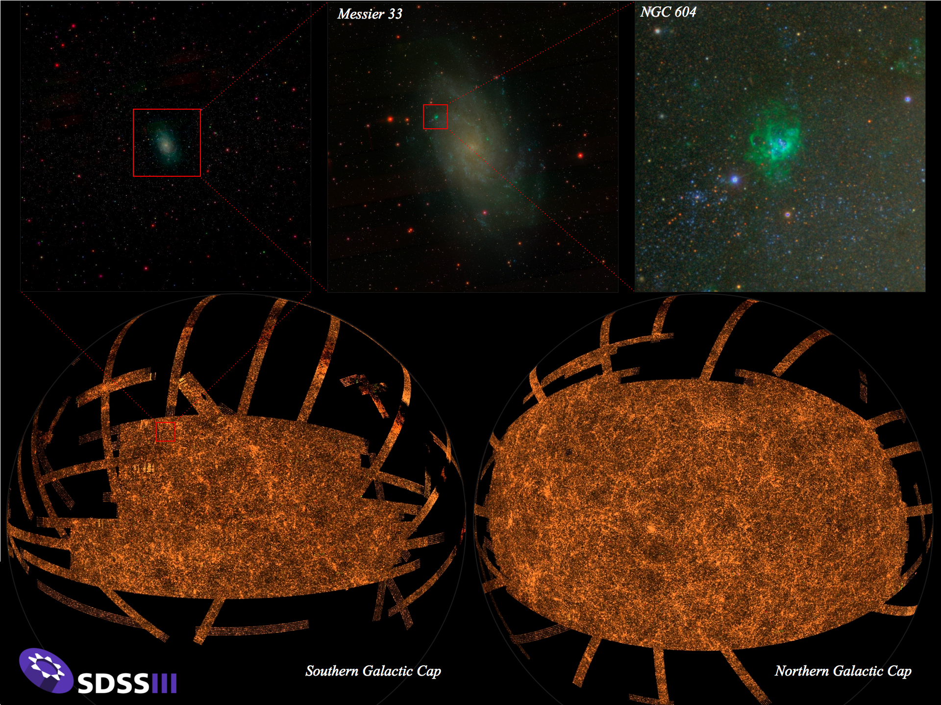
A map of the Universe from SDSS where the distance to galaxies is given in terms of their redshift. Credit: SDSS
In March, we came back to the most local Universe, with a post by SDSS-IV Spokesperson, Jennifer Johnson (Ohio State University) on How SDSS Uses Light to Understand Stars Inside and Out in the Kepler Field. This was about part of the APOGEE survey, which is measuring spectra from stars which have light curves measured by the Kepler Satellite. This is a valuable experiment, as the combination of spectra and light curves allows us to measure the masses, ages and compositions of these stars.

The Kepler Field. Credit: NASA
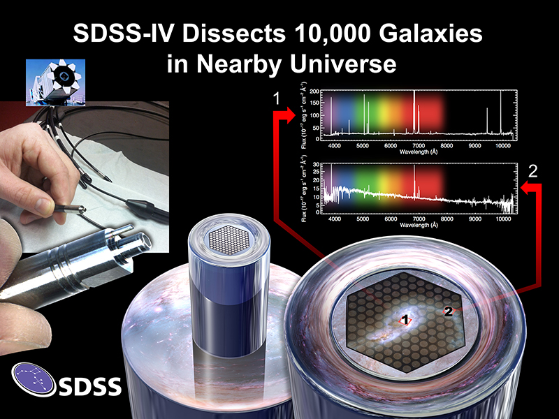
In April, we moved back outside our own Galaxy, to measuring the invisible mass in other galaxies, with a post on How SDSS Uses Light to Explore the Invisible, by the MaNGA Lead Observer, and SDSS-IV Data Release Co-ordinator, Anne-Marie Weijmans from St Andrew University. This post talked about how MaNGA is measuring spectra across the face of nearby galaxies in order to get measurements of the internal motions (again using the redshift/blueshift of the spectra). These measurements give a way to measure the total mass of galaxies, which we find in all cases is much much more than the mass in stars.

For May we went back in the history of SDSS, and talked about How SDSS Used Light to Make the Largest Ever Digital Image of the Night Sky. This post was about the the SDSS camera and the SDSS imaging survey, which ran from 2000-2008, and created a image of over 30% of the sky, containing over a trillion pixels (an image which dwarfs others that have also been claimed as the largest).

The SDSS Camera, now in storage in the Smithsonian Museum. Credit: SDSS, Xavier Poultney
June also saw a post about SDSS imaging, and about an unexpected use for them, finding asteroids, in How SDSS Uses Light to Find Rocks in Space. This has been beautiful visualized in the below video, by Alex Parker.
If our posts in February, March and April confused you because you didn’t understand what astronomers mean by measuring spectra, then the July post was for you: “How SDSS Splits Light into a Rainbow for Science”. This post explained all about what spectra are, how to create them with gratings, and contained a with bonus activity to make your own spectroscope created by the SDSS Education and Public Outreach group.

Comparison of the spectra obtained from a diffraction grating by diffraction (1), and a prism by refraction (2).Credit: Wikimedia
Our August post, by the APOGEE survey Public Engagement officer, David Whelan (from Austin College, Texas) was about the basic physics of the most abundant element in the Universe (hydrogen): “How SDSS Uses Light to Study the Most Abundant Element in the Universe.”
For September, we visited an IYL2015 Exhibit in Dresden with Zach Pace, Graduate Student at the University of Wisconsin, Madison. Zach reported on SDSS plates on display in the exhibit, linking back to an earlier post in which we explain why we need all these big aluminium plates to do our spectroscopic survey. IYL2015 – SDSS Plates (in Retirement).

SDSS Plate on Exhibit in Dresden.
We went back to the APOGEE survey in October, with a post by Gail Zasowski (from John’s Hopkins University) on How SDSS uses mysterious “missing” light to map the interstellar medium. In this post we learned about how SDSS has helped shed light on the the mystery of missing light caused by absorption in the material which is found between stars in our own Galaxy.
Finally last month, we talked about How SDSS Uses Light to Measure the Mass of Stars in Galaxies. Looking back to the post in February, we claimed that the total mass of galaxies is always much much more than the mass we can count in their stars. But how do we know how much mass is in the stars in a galaxy? This post explains how that can be done using measurements of the light from galaxies.
So that wraps up a year of the celebration of light in the SDSS. We certainly haven’t covered all the ways in which SDSS astronomers are using light to learn about the Universe around us, from asteroids in the solar system, to stars in our own Galaxy and galaxies are the furthest edges of the Universe. But we hope it gives you a flavour for the kinds of things the light collected by SDSS (both images and spectra) can be used for.
If you’re looking for a guided entry into SDSS science (especially suitable for educational use), please visit our Voyages.sdss.org site to discover guided journeys through the Universe. As always all SDSS data (through our 12th public data release, DR12) is available free to download, and look out for DR13 (including the first data from SDSS-IV) coming up in mid 2016.


